Plot gallery

This page contains a collection of plots from the Etna example data. All plots are generated by the example scripts (see Example scripts).

Outputs from the main example scripts

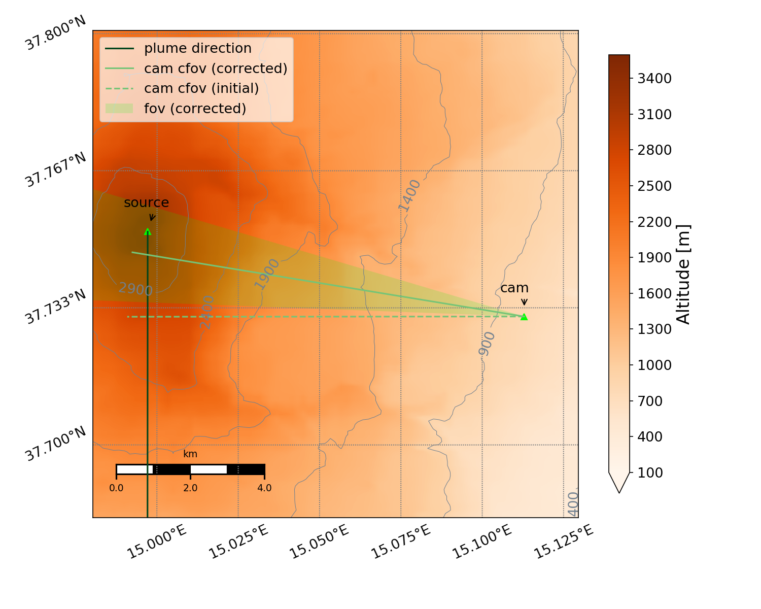
2D map showing a measurement setup (automatically created using class MeasGeometry)

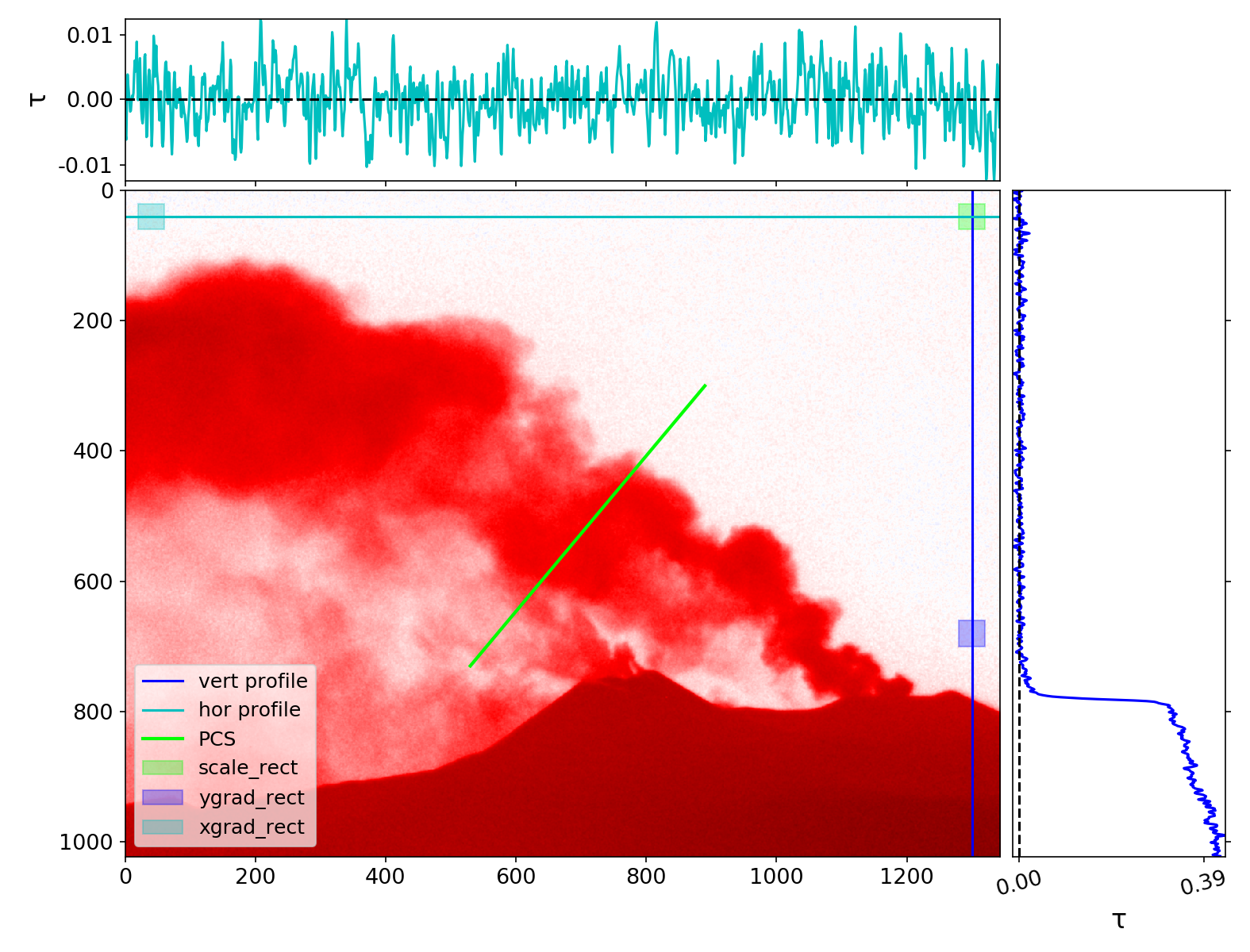
On-band optical density image determined using plume background modelling mode 6 in class PlumeBackgroundModel

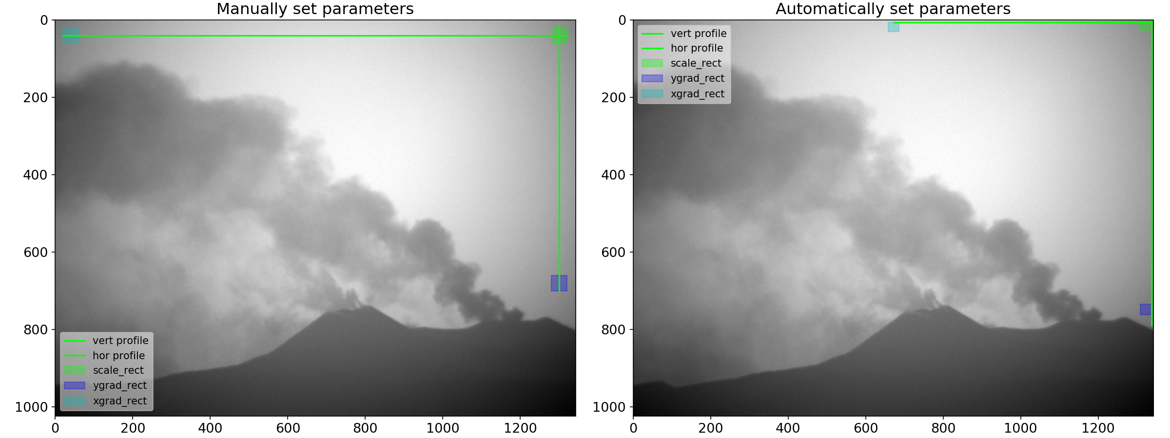
Exemplary sky reference areas for plume background modelling, left: set manually, right: set automatically (cf. example script 3)

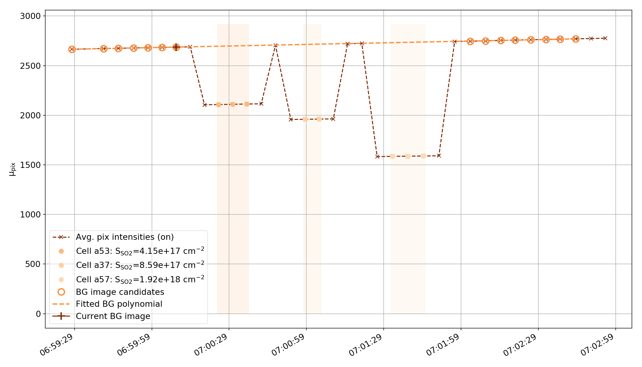
Result of routine for automatic detection of SO2 cell time windows (from time series of on-band images, cf. example script 5)

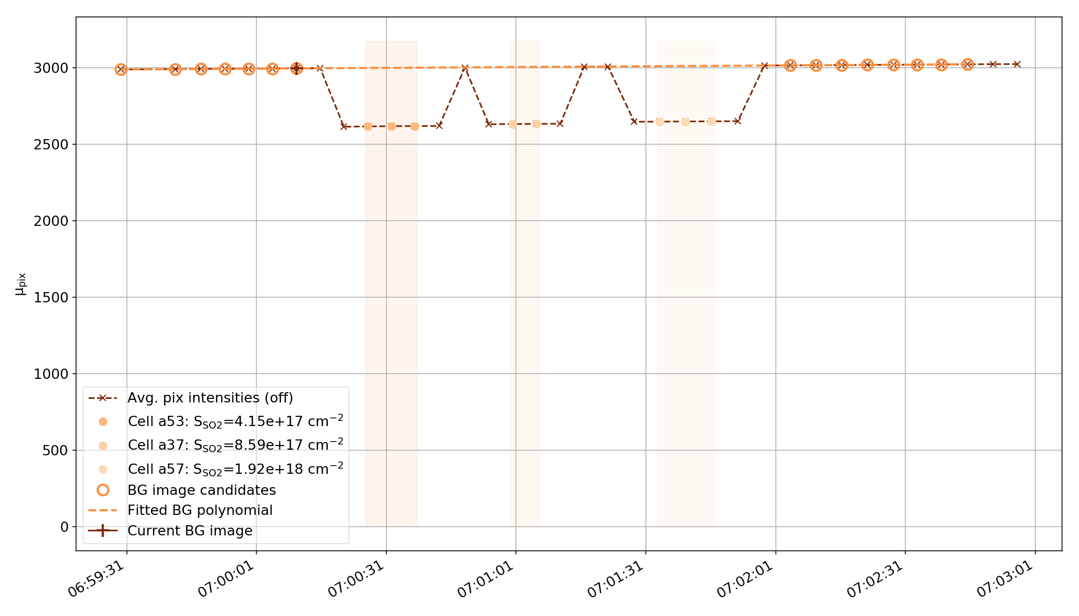
Result of routine for automatic detection of SO2 cell time windows (from time series of off-band images, cf. example script 5)

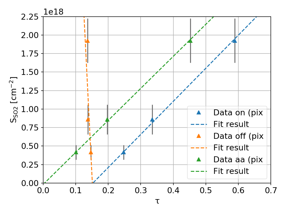
Exemplary SO2 cell calibration curves (for center image pixel, cf. example script 5)

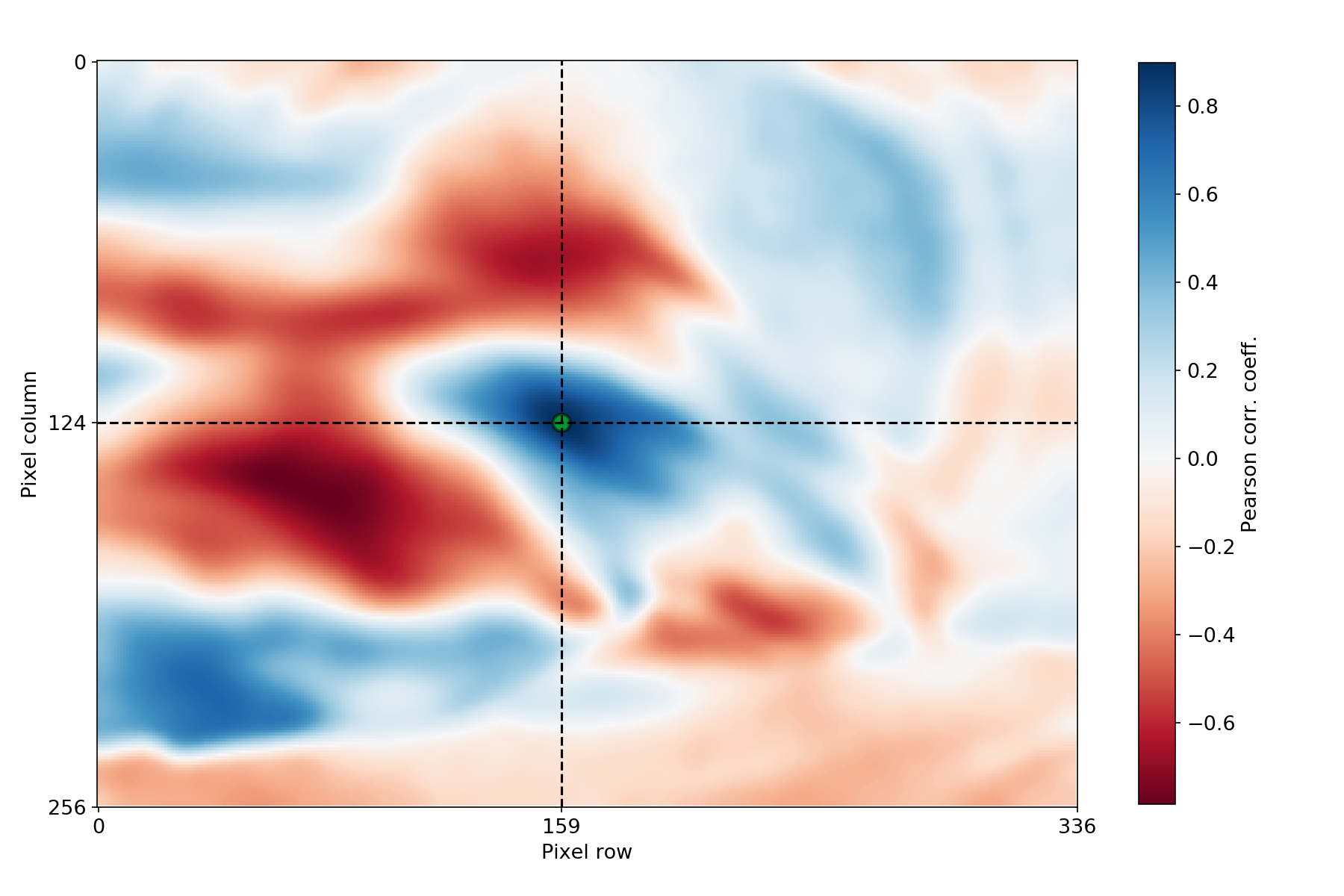
Result of DOAS FOV search using Pearson correlation method (cf. example script 6)

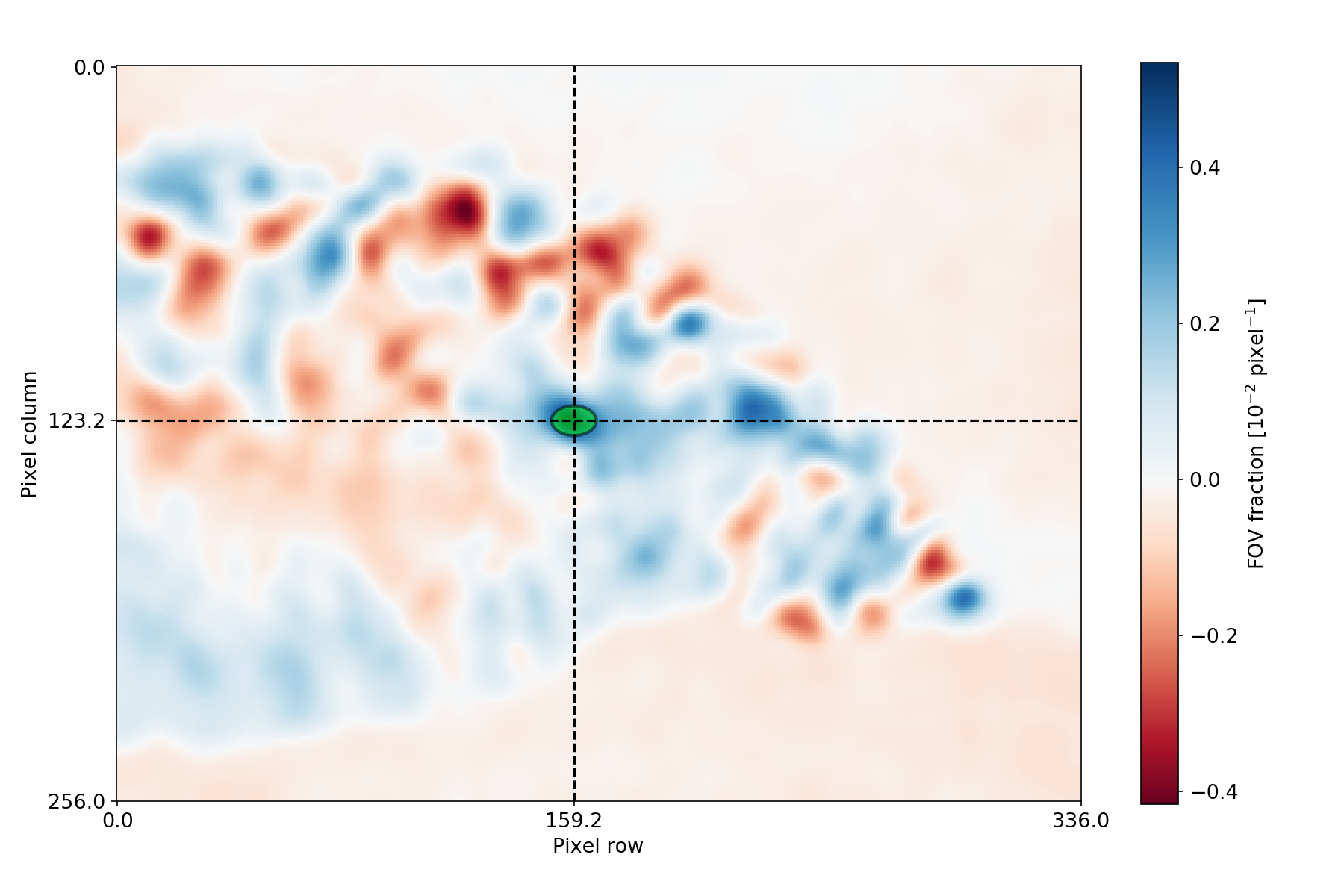
Result of DOAS FOV search using IFR method (cf. example script 6)

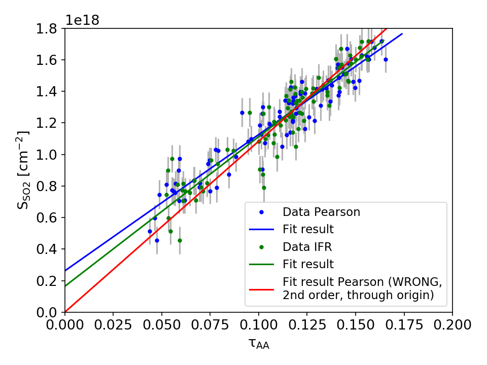
Exemplary DOAS calibration curves determined using the FOV results shown in the prev. 2 Figs. (cf. example script 6)

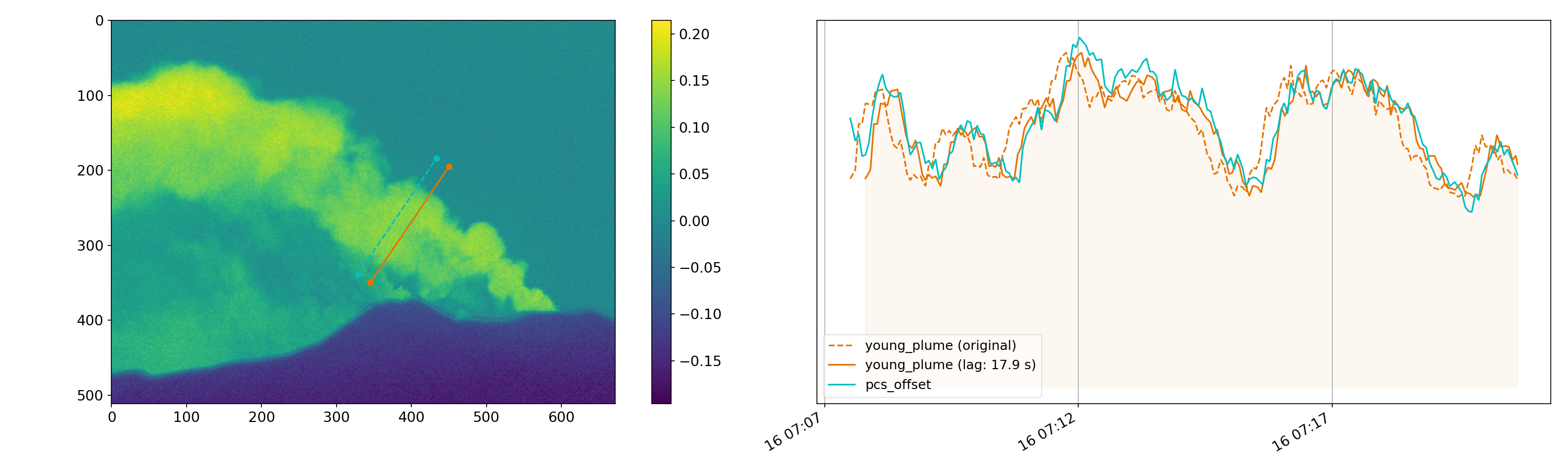
Left: plume AA image including two plume cross section lines used for cross correlation based plume velocity retrieval. Right: Result of cross correlation analysis using the two PCS lines shown left resulting in a velocity of 4.29 m/s (cf. example script 8)

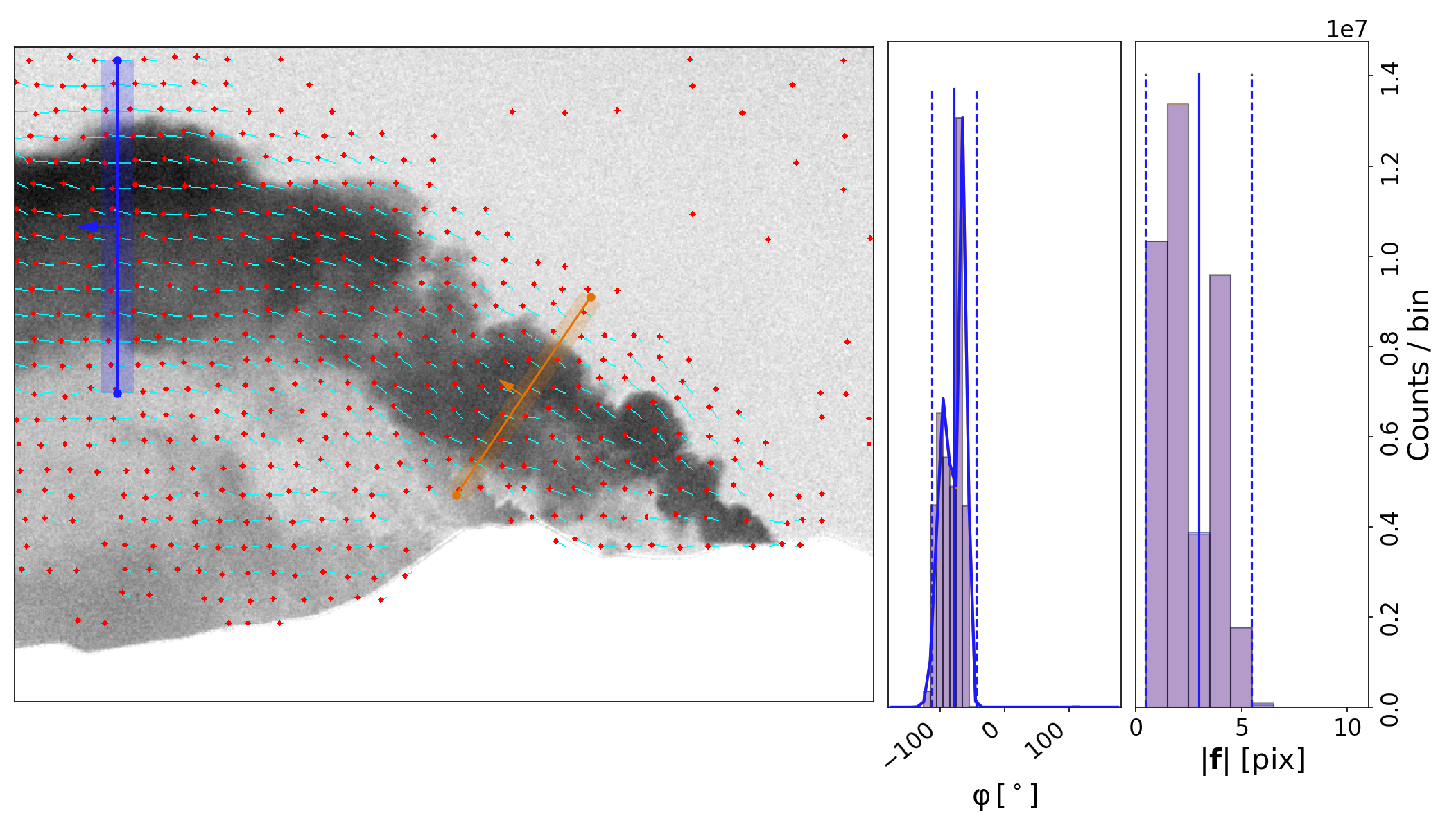
Example output of optical flow Farneback algorithm (left) including histograms of orientation angles (middle) and flow vector magnitudes (right) retrieved within ROIs around both lines. Retrieved expectation values and intervals, derived from 1. and 2. moments of the histograms are indicated by solid and dashed lines, respectively (cf. ex. script 9).

Time series of plume velocity parameters (direction, top; displacement length, bottom) retrieved using histogram based post analysis of optical flow field for the two retrieval lines shown in prev. Fig. (cf. ex. script 9)

SO2-CD image corrected for signal dilution using pixels along terrain features in the images (lime and blue lines) to estimate atmospheric extinction coefficients.

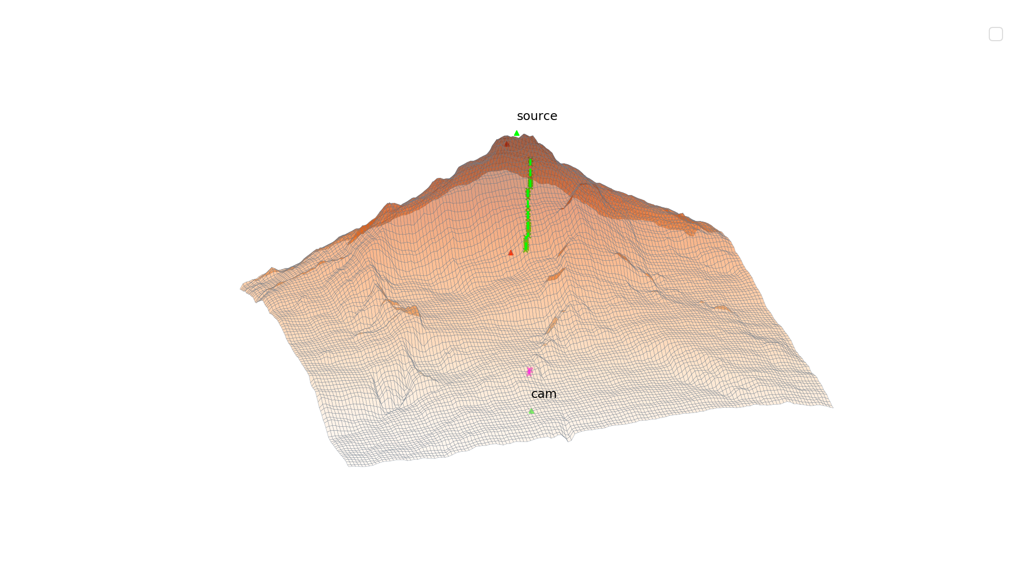
3D map showing results of pixel based distance retrieval to terrain features used for signal dilution correction (cf. prev. Fig.)

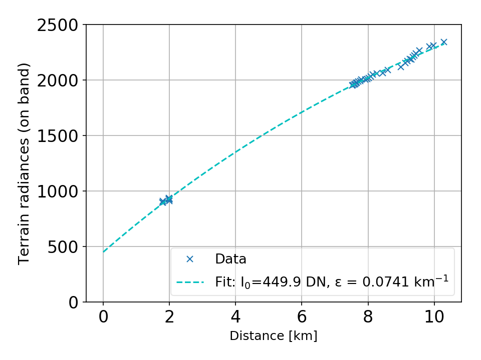
Result of signal dilution correction fit to retrieve atmospheric extinction coefficients (on-band)

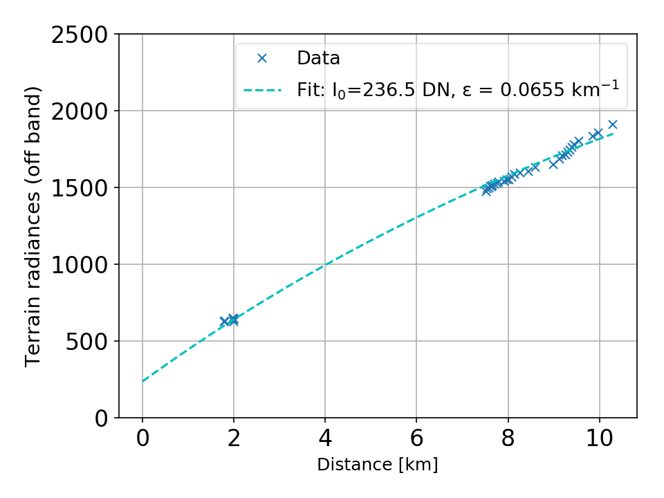
Result of signal dilution correction fit to retrieve atmospheric extinction coefficients (off-band)

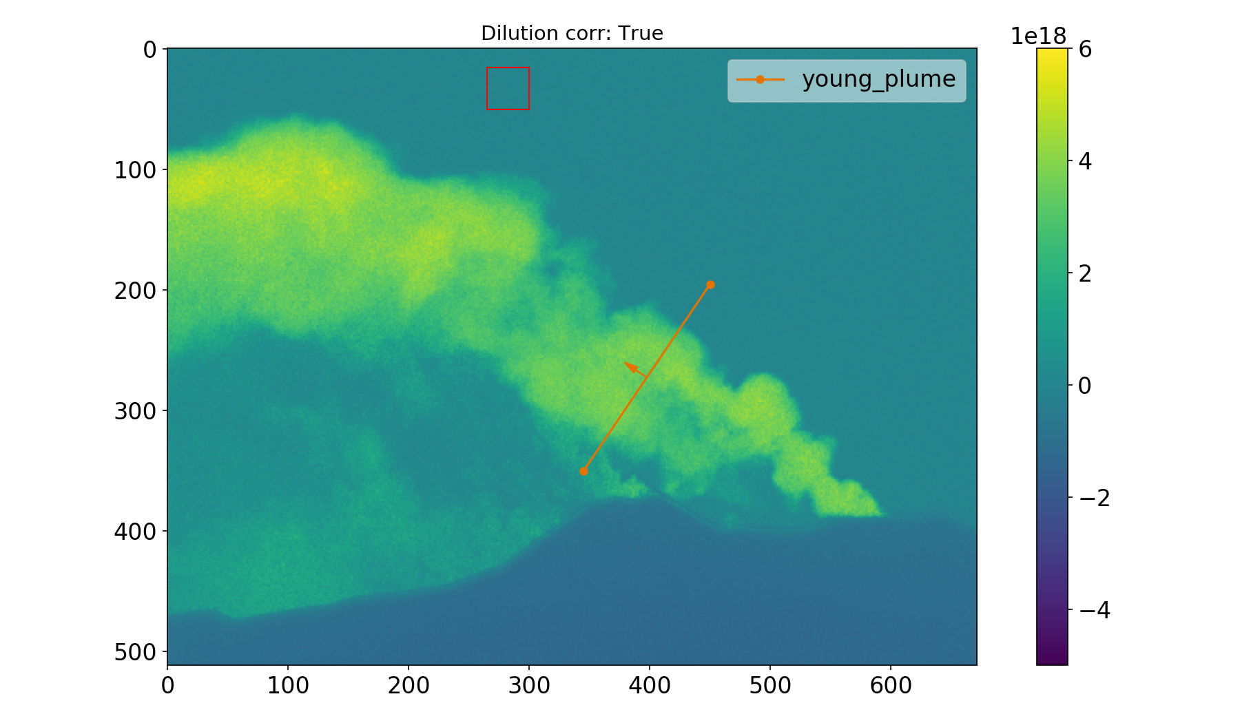
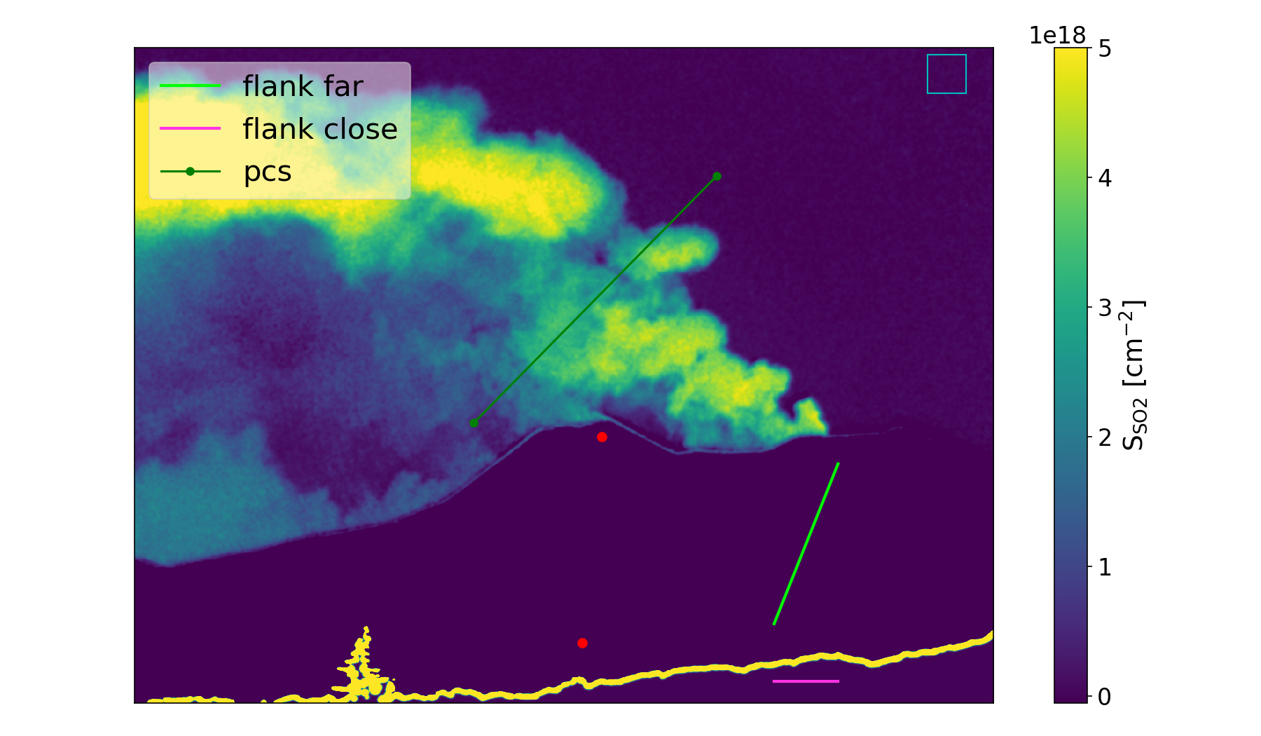
Calibrated SO2-CD image of the Etna plume (not dilution corrected) including retrieval line L (young_plume) and area (red rectangle) used as quality check when performing emission rate analysis (cf. bottom panel, next plot).

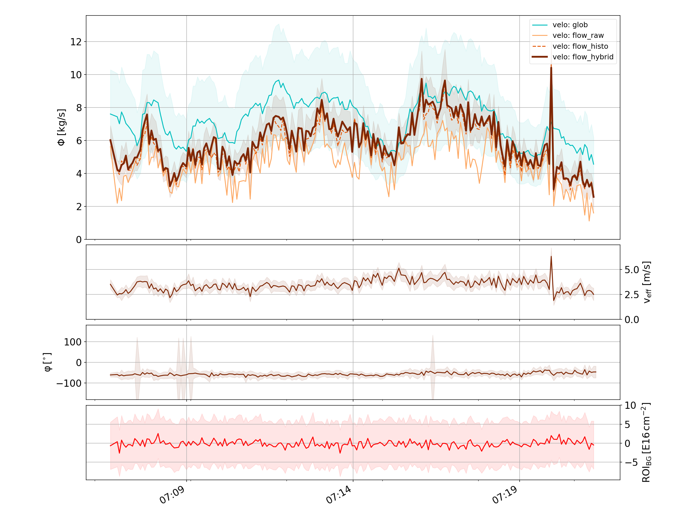
Etna emission rates through L (see prev. Fig) using four different plume velocity retrievals (top, see legend), and velocity results from histogram analysis (2., 3. panel). Bottom: time series of retrieved background CDs in gas free rectangular area (cf. prev. Fig.).

Additional outputs from the introduction scripts

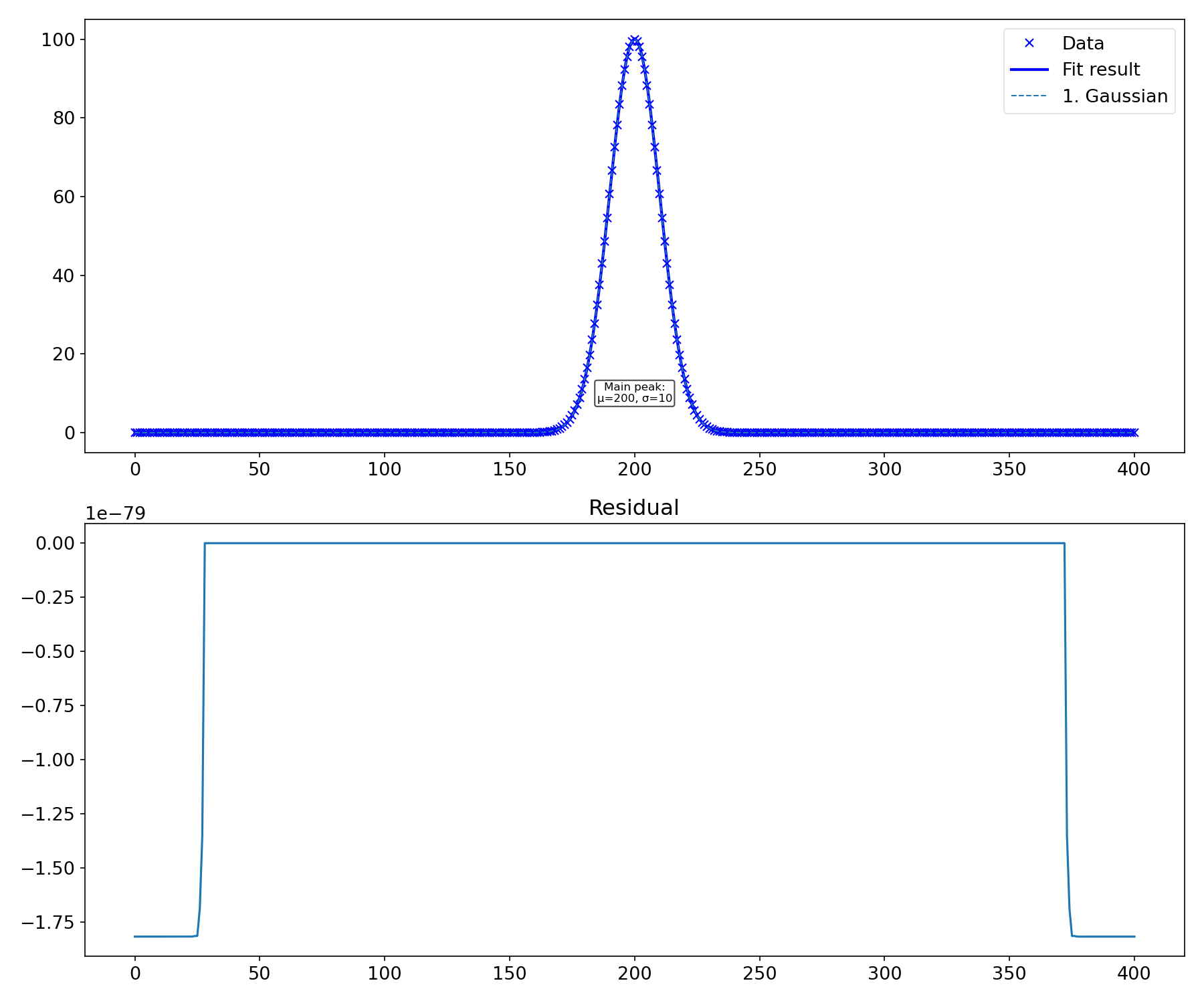
Example output illustrating the pyplis.optimisation.MultiGaussFit class, which is central to the plume velocity retrieval using optical flow methods. This example illustrates the fit result for a signal comprising a single Gaussian.

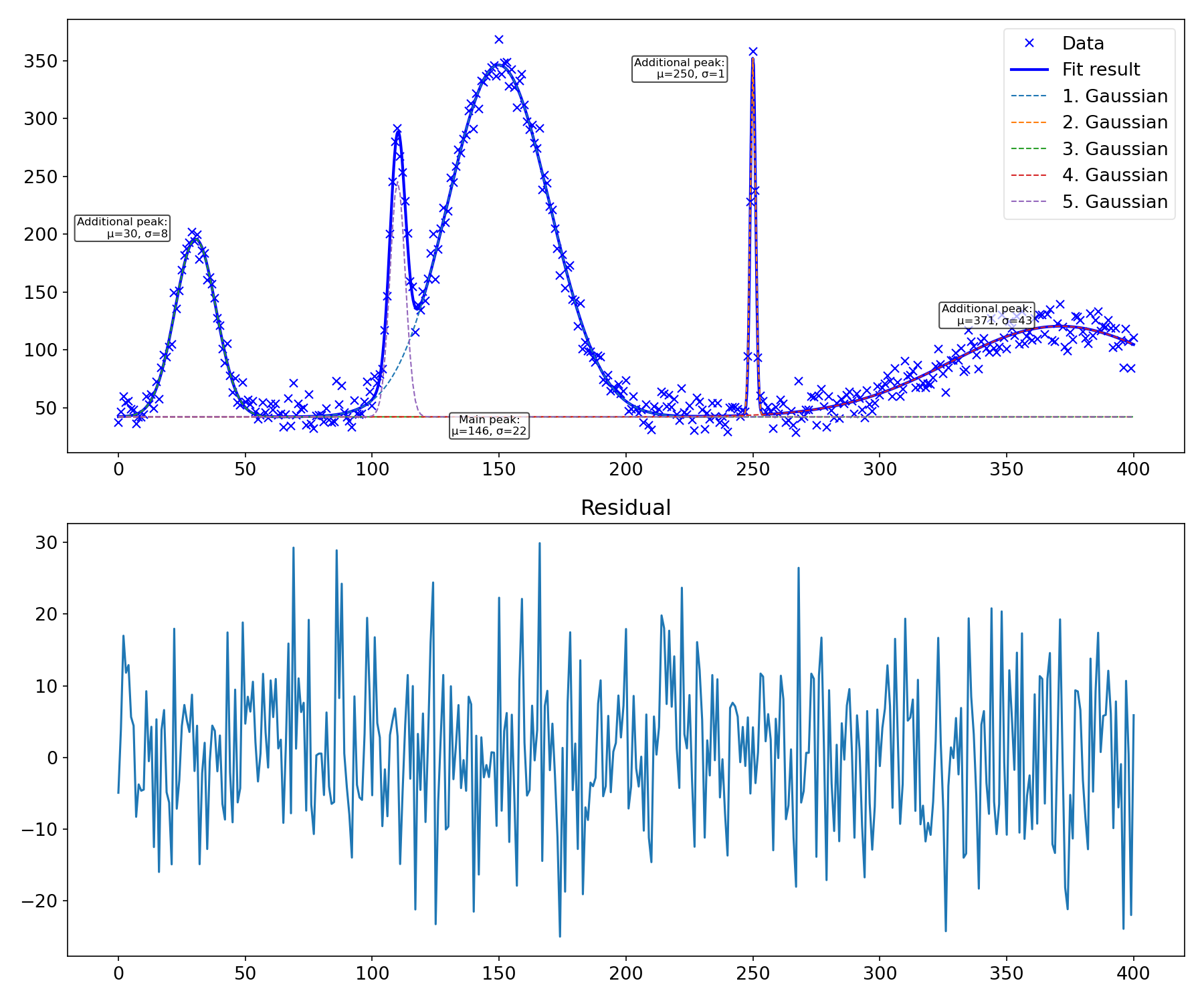
Example output illustrating the pyplis.optimisation.MultiGaussFit class, which is central to the plume velocity retrieval using optical flow methods. This example illustrates the fit result for a more complex signal comprising multiple distinct as well as partially overlapping Gaussians.